Optimization in Deep Learning

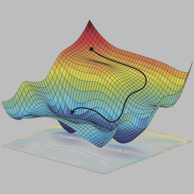
Optimizers are essential components of machine learning algorithms, responsible for adjusting the parameters of a model to minimize the loss function. A loss function measures how well the model’s predictions match the true values, and the optimizer helps find the parameters (weights) that minimize this loss. Essentially, the optimizer guides the model to find the optimal set of weights that result in the best performance.

In this blog post, we will dive into the basics of some popular optimizers used in machine learning: Stochastic Gradient Descent (SGD), SGD with Momentum, and Adam. We will also visualize how each of these optimizers performs in finding the minimum of a given loss curve.

Stochastic Gradient Descent

SGD is a variation of gradient descent where the model parameters are updated using a random subset (mini-batch) of the training data, rather than the full dataset. Optimization in Deep Learning 8bb36e402f474b5dafc670b954531141 The basic update rule for SGD is:

w = w - η∇L(w)

where:

w represents the model parameters (weights),
η is the learning rate,
∇L(w) is the gradient of the loss function L(w) with respect to the weights w.

SGD with Momentum

Momentum is an extension to SGD that helps accelerate the gradient descent by considering the previous gradient updates. It introduces a “momentum” term, which accumulates the gradients over time, making the optimizer less sensitive to noisy updates.

The update rule for

SGD with momentum

is:

                   vₜ = βvₜ₋₁ + (1-β)∇L(w)

                  w = w - ηvₜ

where:

vt is the velocity (momentum) at time step t
β is the momentum coefficient (typically between 0 and 1)
vt-1 is the previous velocity

Adam (Adaptive Moment Estimation)

Adam is an advanced optimizer that combines ideas from both Momentum and RMSProp (Root Mean Square Propagation). It adapts the learning rate for each parameter by maintaining an exponentially decaying average of past gradients and squared gradients.

The update rules for Adam are:

mₜ = β₁mₜ₋₁ + (1 - β₁)∇L(w)

vₜ = β₂vₜ₋₁ + (1 - β₂)(∇L(w))²

m̂ₜ = mₜ/(1 - β₁ᵗ), v̂ₜ = vₜ/(1 - β₂ᵗ)

w = w - η(m̂ₜ/√v̂ₜ + ε)

where:

mₜ is the first moment estimate (mean of the gradients),
vₜ is the second moment estimate (mean of the squared gradients),
m̂ₜ and v̂ₜ are bias-corrected estimates
β₁ and β₂ are the decay rates for the moment estimates (typically set to 0.9 and 0.999, respectively)

Visualizing the Optimizer performance

First we import the necessary packages.

import numpy as np
## PyTorchimport torch
import torch.nn as nn
import torch.nn.functional as F
import torch.utils.data as data
import torch.optim as optim
## Imports for plottingimport matplotlib.pyplot as plt
from matplotlib import cm
import seaborn as sns

In order to define our Optimizer Classes, we first define the Base class then we would use inheritance to build sub classes as per our requirements. Beginning with OptimizerTemplate

class OptimizerTemplate:
    def __init__(self, params, lr):
        self.params = list(params)
        self.lr = lr
    def zero_grad(self):
        ## Set gradients of all parameters to zero        for p in self.params:
            if p.grad is not None:
                pgrad.detach_()
                
           # Detaches the gradient tensor from the computational graph.                                   # This is important for some optimizers
				         p.grad.zero_()  
				         
				            
    @torch.no_grad()              # ensures that the setp method runs without tracking operations in the comp graph    
    
    def step(self):
        ## Apply update step to all parameters        
        for p in self.params:
            if p.grad is None: # We skip parameters without any gradients                continue            
            self.update_param(p)
            
            
    def update_param(self, p):
        # To be implemented in optimizer-specific classes        # placeholder method for subclass implementation        
        raise NotImplementedError

class SGD(OptimizerTemplate):
    def __init(self,params,lr):
        super().__init__(params,lr)
    def update_param(self,p):
        p_update =  - self.lr * p.grad
        p.add_(p_update) # equivalent to p = p + p_update, with p direclty add to p  (but no temp variable created to assign sum to p)                        # avoid graph extension and is memory efficient.

In-place operations in Python modify the data directly, rather than creating a new object with the updated data. These operations typically use less memory since they modify the original object without allocating additional space.

class SGDMomentum(OptimizerTemplate):
    def __init__(self, params, lr, momentum=0.0 ):
        super().__init__(params,lr)
        self.momentum = momentum
        self.param_momentum = {p: torch.zeros_like(p.data) for p in self.params} #dictionary to store m_t    def update_param(self, p):
        self.param_momentum[p] = (1 - self.momentum) * p.grad + self.momentum * self.param_momentum[p]
        p_update = -self.lr * self.param_momentum[p]
        p.add_(p_update)

class Adam(OptimizerTemplate):
    def __init__(self, params, lr, beta1=0.9, beta2=0.999, eps=1e-8):
        super().__init__(params, lr)
        self.beta1 = beta1
        self.beta2 = beta2
        self.eps = eps
        self.param_step = {p: 0 for p in self.params} # Remembers "t" for each parameter for bias correction        self.param_momentum = {p: torch.zeros_like(p.data) for p in self.params}
        self.param_2nd_momentum = {p: torch.zeros_like(p.data) for p in self.params}
    def update_param(self, p):
        self.param_step[p] += 1        self.param_momentum[p] = (1 - self.beta1) * p.grad + self.beta1 * self.param_momentum[p]
        self.param_2nd_momentum[p] = (1 - self.beta2) * (p.grad)**2 + self.beta2 * self.param_2nd_momentum[p]
        bias_correction_1 = 1 - self.beta1 ** self.param_step[p]
        bias_correction_2 = 1 - self.beta2 ** self.param_step[p]
        p_2nd_mom = self.param_2nd_momentum[p] / bias_correction_2
        p_mom = self.param_momentum[p] / bias_correction_1
        p_lr = self.lr / (torch.sqrt(p_2nd_mom) + self.eps)
        p_update = -p_lr * p_mom
        p.add_(p_update)

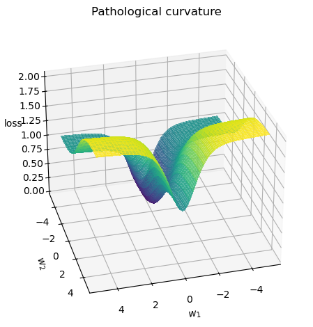
In this notebook, we will visualize the performance of each of these optimizers (SGD, SGD with Momentum, and Adam) on a pathological loss function. This function has been deliberately designed to have a challenging optimization surface, helping us see how each optimizer navigates toward the minimum. We’ll track the trajectories of the optimization process for each optimizer and observe how they behave in their search for the minimum.

def pathological_curve_loss(w1, w2):
    # Example of a pathological curvature. There are many more possible, feel free to experiment here!
    x1_loss = torch.tanh(w1)**2 + 0.01 * torch.abs(w1)
    x2_loss = torch.sigmoid(w2)
    return x1_loss + x2_loss

def plot_curve(curve_fn, x_range=(-5,5), y_range=(-5,5), plot_3d=False, cmap=cm.viridis, title="Pathological curvature"):
    fig = plt.figure()
    ax = plt.axes(projection='3d') if plot_3d else plt.axes()
    x = torch.arange(x_range[0], x_range[1], (x_range[1]-x_range[0])/100.)
    y = torch.arange(y_range[0], y_range[1], (y_range[1]-y_range[0])/100.)
    x, y = torch.meshgrid(x, y, indexing='xy')
    z = curve_fn(x, y)
    x, y, z = x.numpy(), y.numpy(), z.numpy()
    if plot_3d:
        ax.plot_surface(x, y, z, cmap=cmap, linewidth=1, color="#0100", antialiased=False, alpha=0.7)
        ax.view_init(elev=30, azim=75)  # elev (elevation), azim (azimuthal angle)        ax.set_zlabel("loss")
    else:
        ax.imshow(z[::-1], cmap=cmap, extent=(x_range[0], x_range[1], y_range[0], y_range[1]))
    plt.title(title)
    ax.set_xlabel(r"$w_1$")
    ax.set_ylabel(r"$w_2$")
    plt.tight_layout()
    return ax
sns.reset_orig()
_ = plot_curve(pathological_curve_loss, plot_3d = True)
plt.show()

def train_curve(optimizer_func, curve_func=pathological_curve_loss, num_updates=1000, init=[7,7]):
    """
    Inputs:
        optimizer_func - Constructor of the optimizer to use. Should only take a parameter list
        curve_func - Loss function (e.g. pathological curvature)
        num_updates - Number of updates/steps to take when optimizing
        init - Initial values of parameters. Must be a list/tuple with two elements representing w_1 and w_2
    Outputs:
        Numpy array of shape [num_updates, 3] with [t,:2] being the parameter values at step t, and [t,2] the loss at t.
    """
    weights = nn.Parameter(torch.FloatTensor(init), requires_grad=True)
    optimizer = optimizer_func([weights]) # defines parameters to update after the grad calculation

    list_points = []
    for _ in range(num_updates):
        loss = curve_func(weights[0], weights[1])
        list_points.append(torch.cat([weights.data.detach(), loss.unsqueeze(dim=0).detach()], dim=0))
        optimizer.zero_grad()
        loss.backward()
        optimizer.step()
    points = torch.stack(list_points, dim=0).numpy()   # combines list of tensors into a single 2D tensort. 
    return points

The torch.stack() function is used to concatenate a list of tensors along a new dimension, creating a 2D array where each row corresponds to the parameters and loss at a given optimization step. This is particularly useful when we need to visualize or analyze the entire optimization process later on, such as in tracking how the optimizer navigates through the loss landscape. For example consider the following tensor arrangement as list_points

list_points = [
    torch.tensor([5.0, 5.0, 1.2]),  # Step 0: w1=5.0, w2=5.0, loss=1.2
    torch.tensor([4.5, 4.2, 1.0]),  # Step 1: w1=4.5, w2=4.2, loss=1.0
    torch.tensor([4.0, 3.8, 0.8])   # Step 2: w1=4.0, w2=3.8, loss=0.8
]

The torch.stack() would return stacked form of each from list to a single tensor as below:

tensor([[5.0000, 5.0000, 1.2000],
        [4.5000, 4.2000, 1.0000],
        [4.0000, 3.8000, 0.8000]]

In terms of optimization, we can imagine that w1w1 and w2 are the weight parameters, and the curvature represents the loss surface over the space of these weights. In typical neural networks, however, we deal with many more parameters, and the loss surface can become much more complex and multi-dimensional. Nevertheless, the core concepts of optimization remain the same.

Ideally, our optimization algorithm would find the center of the ravine in the loss surface, where the gradient is steepest, and focus on optimizing the parameters towards the direction of the minimum. However, if the optimizer encounters a point along the ridges of the curvature, the gradient is much greater in one direction (say, w1) than in the other (w2). This can cause the optimizer to jump from one side of the ridge to the other, causing instability. Due to these large gradients, the optimizer might need to reduce its learning rate, significantly slowing down the learning process.

Visualizing working of different algorithms

At first, lets take a 50 iteration to see the performance of SGD, SGD with Momentum and ADAM optimizer. We set higher learning rate for algorithm. This is because we only have 2 parameters instead of tens of thousands or even millions.

SGD_points = train_curve(lambda params: SGD(params, lr=10),num_updates=50)
SGDMom_points = train_curve(lambda params: SGDMomentum(params, lr=10, momentum=0.9),num_updates=50)
Adam_points = train_curve(lambda params: Adam(params, lr=1),num_updates=50)

To understand best how the different algorithms worked, we visualize the update step as a line plot through the loss surface. We will stick with a 2D representation for readability.


# Visualise the working of different algorithmsall_points = np.concatenate([SGD_points, SGDMom_points, Adam_points], axis=0)
ax = plot_curve(pathological_curve_loss,
                x_range=(-np.absolute(all_points[:,0]).max(), np.absolute(all_points[:,0]).max()),
                y_range=(all_points[:,1].min(), all_points[:,1].max()),
                plot_3d=False)
ax.plot(SGD_points[:,0], SGD_points[:,1] ,color="red", marker="o", zorder=1, label="SGD")
ax.plot(SGDMom_points[:,0], SGDMom_points[:,1], color="blue", marker="o", zorder=2, label="SGDMom")
ax.plot(Adam_points[:,0], Adam_points[:,1], color="grey", marker="o", zorder=3, label="Adam")
plt.legend()
plt.show()

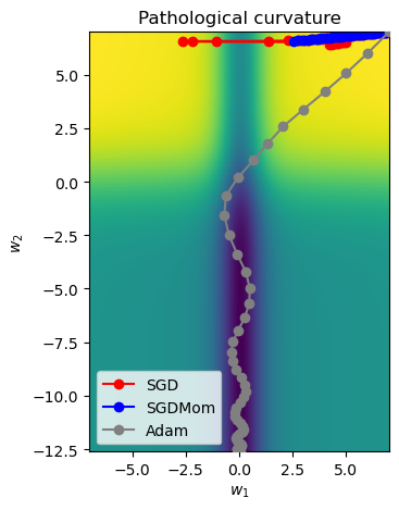
We can observer that the optmizer encounters a point along the ridges of the curvature and cause the optimizer to jump from one side of the ridge to the other, not being able to find the steepest region. While ADAM has been able to do so.

Now we increase iteration to 1000 (default), and observe the performance.


SGD_points = train_curve(lambda params: SGD(params, lr=10))
SGDMom_points = train_curve(lambda params: SGDMomentum(params, lr=10, momentum=0.9))
Adam_points = train_curve(lambda params: Adam(params, lr=1))

# Visualise the working of different algorithms
all_points = np.concatenate([SGD_points, SGDMom_points, Adam_points], axis=0)
ax = plot_curve(pathological_curve_loss,
                x_range=(-np.absolute(all_points[:,0]).max(), np.absolute(all_points[:,0]).max()),
                y_range=(all_points[:,1].min(), all_points[:,1].max()),
                plot_3d=False)
ax.plot(SGD_points[:,0], SGD_points[:,1] ,color="red", marker="o", zorder=1, label="SGD")
ax.plot(SGDMom_points[:,0], SGDMom_points[:,1], color="blue", marker="o", zorder=2, label="SGDMom")
ax.plot(Adam_points[:,0], Adam_points[:,1], color="grey", marker="o", zorder=3, label="Adam")
plt.legend()
plt.show()

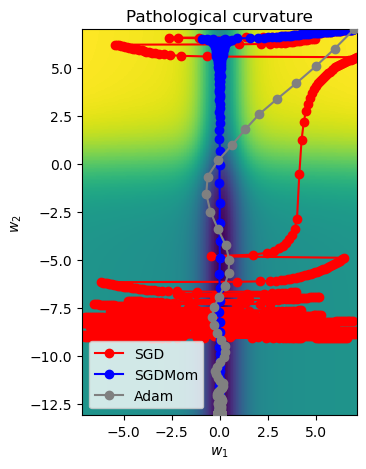
The observations can be made as:

SGD (Stochastic Gradient Descent): struggles due to the curvature, leading to erratic and slow progress toward the minima.
SGDMom (SGD with Momentum): smooths the updates by accumulating velocity, allowing for faster progress and less oscillation.
Adam: it adjusts the learning rate for each parameter dynamically, resulting in a stable and direct path to the minima.

After examining the performance of various optimizers like SGD, SGD with momentum, and Adam, it’s tempting to think that Adam is always the best choice due to its faster convergence and ability to handle sparse gradients effectively. However, the answer is not so straightforward. While Adam has become the go-to optimizer in many deep learning tasks due to its adaptive learning rate and efficiency, it doesn’t always outperform SGD, especially in terms of generalization.

Why not always Adam?

Overfitting and Generalization: One of the key observations is that Adam can sometimes overfit the training data. This is because Adam, due to its adaptive learning rate, tends to make more aggressive updates early in the training and can get stuck in sharp minima of the loss surface. Sharp minima are often correlated with models that overfit on the training data, meaning they perform well on the training set but poorly on unseen data (test set).

On the other hand, SGD with momentum tends to find “wider” optima — regions of the loss surface that are flatter. Wider minima have been shown to correspond to models that generalize better, meaning they are less likely to overfit. This phenomenon is related to the concept of generalization error: models that converge to flatter minima are less sensitive to small fluctuations in the training data, making them more robust when applied to unseen data.
Practical Considerations:
- Training Time: Adam often converges faster than SGD due to its adaptive learning rate, which makes it a good choice when training on complex models or when time is a constraint. However, in some cases, the faster convergence might be at the cost of overfitting, as mentioned earlier.
- Stability and Robustness: SGD with momentum, although slower, is more stable and tends to provide better performance on a wider range of problems, especially in settings where the training data is noisy or when a high degree of generalization is needed.

Conclusion

Optimizers are critical to training deep learning models efficiently and effectively. The choice of optimizer can significantly impact the training speed and final model performance. By visualizing the behavior of different optimizers, we can better understand their strengths and how they navigate complex loss landscapes.

In summary, the choice of optimizer depends on the task at hand. It’s worth experimenting with both Adam and SGD (with momentum) to see which works best for a given problem. And while Adam is a great default choice for many tasks, it’s important not to overlook the benefits of SGD, especially when generalization is a top priority.

Stochastic Gradient Descent#

SGD with Momentum#

Adam (Adaptive Moment Estimation)#

Visualizing the Optimizer performance#

Visualizing working of different algorithms#

Why not always Adam?#

Conclusion#

Stochastic Gradient Descent

SGD with Momentum

Adam (Adaptive Moment Estimation)

Visualizing the Optimizer performance

Visualizing working of different algorithms

Why not always Adam?

Conclusion