1. Introduction to RAG Fundamentals

Hey everyone, and welcome to our deep dive into Retrieval-Augmented Generation, or RAG! In the rapidly evolving world of Large Language Models (LLMs), we’ve seen incredible feats of text generation, translation, and conversation. However, even the most powerful LLMs have limitations. They can sometimes “hallucinate” – producing plausible but incorrect information – or lack knowledge about events that occurred after their training data was collected.

The Core Problem: Standard LLMs generate responses based solely on the patterns learned during their massive training phase. Their knowledge is essentially frozen at a point in time and limited to the data they were trained on. How can we make them more knowledgeable about specific domains, recent events, or private data without expensive retraining?

Enter RAG: Retrieval-Augmented Generation is an architectural approach that bridges this gap. Instead of relying only on its internal knowledge, a RAG system first retrieves relevant information from an external knowledge source (like a collection of documents, a database, or specific websites) before generating a response. This retrieved information is then used as context by the LLM to craft a more accurate, timely, and relevant answer.

How does it work? The Basic Flow:

1. Query Input: The user provides a prompt or question.
2. Retrieval: The system searches a pre-defined knowledge base (often vectorized documents stored in a vector database) to find chunks of text that are semantically relevant to the user’s query.
3. Augmentation: The original query and the retrieved text snippets are combined into a new, augmented prompt. This prompt essentially instructs the LLM to answer the query using the provided context.
4. Generation: The LLM receives the augmented prompt and generates the final response, grounding its answer in the retrieved information.

Why RAG? Key Benefits:

• Improved Accuracy & Reduced Hallucinations: By grounding responses in real data, RAG significantly reduces the chance of the LLM making things up.
• Access to Timely Information: RAG systems can access up-to-date knowledge bases, overcoming the “knowledge cutoff” problem of static LLMs.
• Domain Specificity: Easily adapt LLMs to specific domains (e.g., legal, medical, internal company documents) without fine-tuning the entire model.
• Transparency & Explainability: You can often trace why the LLM gave a specific answer by looking at the retrieved documents.
• Cost-Effective: Often more efficient than constantly retraining or fine-tuning massive models for new information.

Core Components (A Sneak Peek):

Throughout this series, we’ll explore the key building blocks of a RAG system:

• The Knowledge Base: Your collection of documents or data.
• Text Processing: Chunking and preparing your data.
• Embeddings: Numerical representations of your text’s meaning.
• Vector Database: Storing and efficiently searching embeddings.
• The Retriever: The mechanism for finding relevant context.
• The Generator (LLM): The language model that crafts the final answer.

Stay tuned as we dive deep into each of these components, starting with how we prepare our text data for effective retrieval in the next sectio!

2. Text Processing Deep Dive

In our introduction, we established that RAG systems retrieve information from an external knowledge base. But how do we get our raw documents – PDFs, web pages, text files – into a format suitable for efficient retrieval? This is where text processing comes in, and it’s a critical foundation for any successful RAG pipeline.

Why Process Text?

Raw text is unstructured. Computers, especially the embedding models used in RAG, work best with smaller, manageable units of text. Furthermore, the quality of retrieval heavily depends on how well our text is segmented and cleaned. Our goal is to create meaningful “chunks” of information that can be effectively vectorized (turned into embeddings) and later retrieved.

Key Steps in RAG Text Processing:

Loading Data:

Getting the text out of its original format (PDF, HTML, DOCX, TXT, etc.). Libraries like pypdf, beautifulsoup4, python-docx, and standard file I/O are your friends here.

`# Example using pypdf for PDF loading
from pypdf import PdfReader

def load_pdf_text(file_path):
    reader = PdfReader(file_path)
    text = ""
    for page in reader.pages:
        text += page.extract_text() + "\n" # Add newline between pages
    return text

# pdf_text = load_pdf_text("your_document.pdf")
# print(f"Loaded {len(pdf_text)} characters.")

Chunking (Segmentation):

This is arguably the most crucial step. We need to break down large documents into smaller, semantically coherent pieces. If chunks are too small, they might lack context. If they’re too large, they might contain irrelevant information, diluting the signal for retrieval, and potentially exceed the LLM’s context window limit.

• Fixed-Size Chunking: The simplest method. Split text every N characters or tokens. Often uses overlap to ensure context isn’t lost entirely at boundaries.
  • Pro: Easy to implement.
  • Con: Can split sentences or ideas mid-way, harming semantic meaning.
• Recursive Character Text Splitter (Common in LangChain): Tries to split based on a hierarchy of separators (e.g., \n\n, \n, , ``). It recursively splits until chunks are small enough. More robust than simple fixed-size.
• Semantic Chunking: Uses NLP techniques (e.g., sentence embedding similarity, topic modeling) to group related sentences or paragraphs together. Aims for semantically meaningful chunks.
  • Pro: Creates contextually rich chunks.
  • Con: More computationally intensive; effectiveness depends on the NLP model used.
• Sentence Splitting: Splits text into individual sentences (using libraries like nltk or spacy). Often a good starting point before potentially grouping sentences.

# Example using LangChain's RecursiveCharacterTextSplitter
from langchain_text_splitters import RecursiveCharacterTextSplitter

text = "Your long document text goes here..." # Assume 'text' is loaded

# Define splitter parameters
text_splitter = RecursiveCharacterTextSplitter(
    chunk_size=1000,  # Target size in characters
    chunk_overlap=200, # Overlap between chunks
    length_function=len,
    is_separator_regex=False,
    separators=["\n\n", "\n", " ", ""], # Hierarchy of separators
)

chunks = text_splitter.split_text(text)
# print(f"Split text into {len(chunks)} chunks.")
# print(f"Example chunk:\n{chunks[0][:200]}...") # Print start of first chunk

Choosing the right chunk size and overlap is crucial and often requires experimentation.

1. Cleaning (Optional but Recommended): Removing noise can sometimes improve embedding quality.

   • Removing Boilerplate: Headers, footers, irrelevant sidebars (especially from web scrapes).
   • Normalization: Lowercasing, removing excessive whitespace.
   • Handling Special Characters: Decide whether to keep or remove them.
   • Caution: Overly aggressive cleaning (like removing all punctuation or stop words) can sometimes harm meaning, especially for sentence-based embedding models. Evaluate the impact.

2. Metadata Extraction: While processing, associate useful metadata with each chunk. This is invaluable later for filtering searches or providing context to the LLM. Examples:

   • Source Filename/URL
   • Page Number
   • Section Header
   • Timestamps
   • Chapter Title

   # Integrating metadata during chunking (conceptual)
   # When creating documents/chunks for LangChain or similar:
   # metadata = {"source": "your_document.pdf", "page": page_num}
   # document_chunk = Document(page_content=chunk_text, metadata=metadata)
   

The Output: The result of this stage is a list of text chunks (often represented as Document objects in frameworks like LangChain), each potentially carrying relevant metadata. These chunks are now ready to be transformed into numerical representations – embeddings – which we’ll cover next

3. Embedding Space Visualization

We’ve processed our text into chunks. The next step in RAG is to convert these text chunks into embeddings – dense numerical vectors that capture semantic meaning. But what are these vectors, and how can we understand the “space” they live in? This section dives into embeddings and how visualization techniques help us grasp their structure and effectiveness.

What are Embeddings?

At their core, embeddings are vector representations of data (in our case, text). An embedding model (often a specialized transformer model like sentence-transformers) takes a piece of text as input and outputs a fixed-size list of numbers (e.g., 384, 768, or 1024 dimensions). The magic lies in the training process: these models are trained such that texts with similar meanings are mapped to vectors that are close together in the high-dimensional embedding space.

• “The cat sat on the mat” might have an embedding close to “A feline rested upon the rug.”
• Both would be relatively far from “The rocket launched into orbit.”

It is very necessary to understand the Sentence transformers which allow the sentences to have a single embedding rather than each words embedding.

At its core, a Sentence Transformer is a modification of pre-trained Transformer models (like BERT, RoBERTa, XLM-R, etc.) specifically designed to create high-quality sentence embeddings. These embeddings are dense vector representations of sentences where sentences with similar meanings are close together in the vector space.

The Problem with Standard Transformers for Sentence Similarity:

Standard Transformer models like BERT were primarily trained for tasks like masked language modeling and next sentence prediction. They produce excellent contextual word embeddings. However, directly using them for sentence similarity by simply averaging the word embeddings or using the output of the [CLS] token often results in suboptimal performance. The resulting sentence embeddings don’t always capture semantic similarity well.

Using BERT for pairwise sentence comparison (feeding two sentences simultaneously into BERT) yields good results but is computationally very expensive. For finding the most similar pair in a set of 10,000 sentences, it would require roughly 50 million comparisons (n*(n-1)/2), which is often infeasible.

1. Sentence Transformer Architecture:

   • Base Transformer Model: It starts with a pre-trained Transformer model (e.g., BERT). This model processes the input sentence and generates contextual embeddings for each token (word or subword).
   • Pooling Layer: This is a crucial addition. After the base model generates token embeddings, a pooling operation is applied to aggregate these token embeddings into a single, fixed-size vector representing the entire sentence. Common pooling strategies include:
     • Mean Pooling: Calculate the element-wise mean of all output token embeddings. This is often the best-performing default.
     • Max Pooling: Take the element-wise maximum over all output token embeddings.
     • CLS Pooling: Simply use the output embedding of the special [CLS] token (which BERT uses for classification tasks). While viable, mean pooling often works better for similarity tasks.

   Result: The output of the pooling layer is the sentence embedding (e.g., a 384, 768, or 1024-dimensional vector).

2. The Key: Fine-tuning Strategy:

   • The real innovation of Sentence Transformers lies in how they are fine-tuned. They are typically trained using a Siamese or Triplet network structure.
   • Siamese Network:
     • Two identical Sentence Transformer networks (sharing the same weights) process two sentences independently.
     • The resulting two sentence embeddings are compared (usually using cosine similarity).
     • The network is trained using labeled sentence pairs (e.g., pairs known to be paraphrases or semantically unrelated). The objective is to make the embeddings of similar sentences closer (high cosine similarity) and embeddings of dissimilar sentences farther apart (low cosine similarity). Datasets like SNLI (Stanford Natural Language Inference) or MultiNLI are often used, treating entailment pairs as similar and contradiction pairs as dissimilar.
   • Triplet Network:
     • Three identical Sentence Transformer networks process an “anchor” sentence, a “positive” (similar) sentence, and a “negative” (dissimilar) sentence.
     • The network is trained using a triplet loss function. The goal is to minimize the distance between the anchor and positive embeddings while maximizing the distance between the anchor and negative embeddings, ensuring a margin between the two.

3. Inference (How You Use It):

   • Once fine-tuned, you feed a single sentence into the Sentence Transformer model.
   • It passes through the base Transformer and the pooling layer.
   • You get a single vector (the sentence embedding) as output.
   • You can pre-compute embeddings for a large corpus of sentences.
   • To find sentences similar to a query sentence, you compute its embedding and then use efficient vector similarity search (like cosine similarity) against the pre-computed embeddings of the corpus. This is computationally much faster than pairwise comparisons with standard BERT.

Moving back to the Embedding space now. So, Why Visualize the Embedding Space?

Embeddings often have hundreds or even thousands of dimensions, making them impossible to visualize directly. However, understanding the structure of this space is crucial for RAG:

• Debugging Retrieval: Are semantically similar chunks actually clustered together? Are unrelated chunks far apart?
• Identifying Outliers: Are some documents completely isolated, potentially indicating processing errors or unique content?
• Understanding Data Distribution: Does your data form distinct clusters? This might inform chunking strategies or metadata filtering.
• Comparing Embedding Models: Visualizing embeddings from different models for the same data can show which one creates better separation or clustering.

The Challenge: Dimensionality Reduction

To visualize high-dimensional embeddings (e.g., 768D) on a 2D or 3D plot, we need to reduce their dimensionality while preserving the essential structure (i.e., keeping nearby points close and distant points far). Common techniques include:

1. Principal Component Analysis (PCA): A linear technique that finds the principal components (axes) that capture the most variance in the data. It projects the data onto a lower-dimensional subspace defined by these components.
   • Pros: Computationally efficient, deterministic.
   • Cons: Linear assumption might not capture complex, non-linear structures well. Assumes variance is the most important aspect to preserve.
2. t-Distributed Stochastic Neighbor Embedding (t-SNE): A non-linear technique particularly good at revealing local structure and clusters. It models similarities between high-dimensional points and low-dimensional points and tries to minimize the divergence between these two distributions.
   • Pros: Excellent at visualizing well-separated clusters.
   • Cons: Computationally intensive (especially for large datasets), results can vary between runs (non-deterministic), focuses on local structure so global distances might not be well preserved. Parameters (perplexity, learning rate) need tuning.
3. Uniform Manifold Approximation and Projection (UMAP): Another non-linear technique, often seen as a good balance between t-SNE and PCA. It’s based on manifold learning and topological data analysis.
   • Pros: Generally faster than t-SNE, often better at preserving global structure alongside local structure, good cluster separation.
   • Cons: Still non-deterministic, parameter tuning needed (n_neighbors, min_dist).

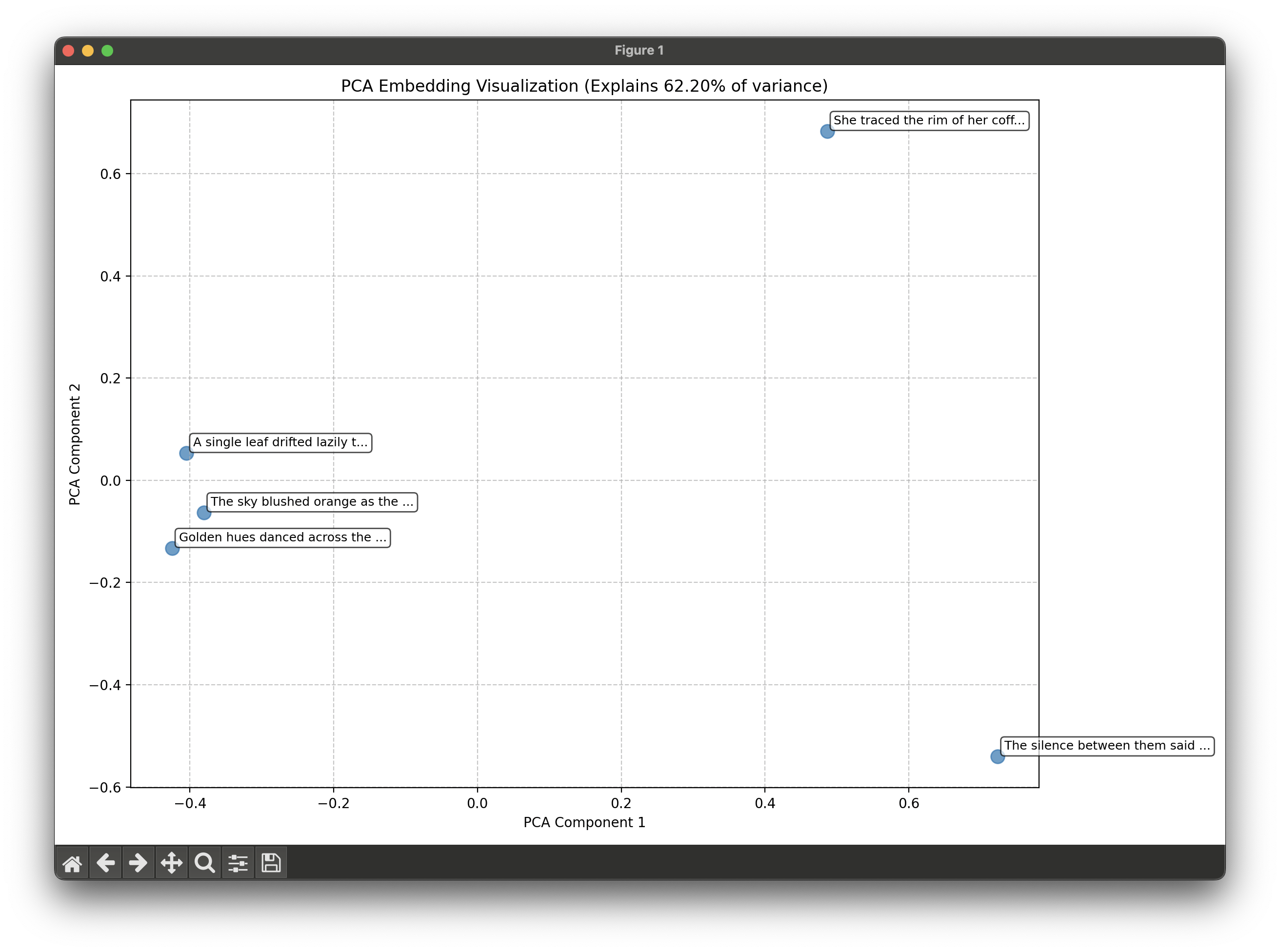
Let’s Visualize!

import numpy as np
from sentence_transformers import SentenceTransformer
from sklearn.decomposition import PCA
import matplotlib.pyplot as plt
import pandas as pd

# Load your data
text_chunks = ["The sky blushed orange as the sun slipped behind the hills.",
"Golden hues danced across the horizon as evening crept in. ",
"She traced the rim of her coffee mug, lost in thought. ",
"A single leaf drifted lazily through the autumn air. ",
"The silence between them said more than any words ever could."]
# Generate embeddings
model = SentenceTransformer('all-MiniLM-L6-v2')
embeddings = model.encode(text_chunks, show_progress_bar=True)
print(f"Generated {len(embeddings)} embeddings of dimension {embeddings[0].shape[0]}")

# PCA dimensionality reduction
pca = PCA(n_components=2)
pca_results = pca.fit_transform(embeddings)
explained_variance = pca.explained_variance_ratio_.sum() * 100
print(f"PCA explains {explained_variance:.2f}% of variance")

# Create DataFrame for plotting
df = pd.DataFrame({
    'PCA_1': pca_results[:, 0],
    'PCA_2': pca_results[:, 1],
    'Text': [t[:30] + "..." if len(t) > 30 else t for t in text_chunks]
})

# Plot
plt.figure(figsize=(12, 8))
plt.title(f"PCA Embedding Visualization (Explains {explained_variance:.2f}% of variance)")
plt.scatter(df['PCA_1'], df['PCA_2'], s=100, alpha=0.7)

# Add labels to some points
n_samples = len(df)
step = max(1, n_samples // 10)  # Show ~10 labels
for i in range(0, n_samples, step):
    plt.annotate(
        df['Text'].iloc[i],
        (df['PCA_1'].iloc[i], df['PCA_2'].iloc[i]),
        fontsize=9,
        xytext=(5, 5),
        textcoords='offset points',
        bbox=dict(boxstyle="round", fc="white", alpha=0.7)
    )

plt.xlabel("PCA Component 1")
plt.ylabel("PCA Component 2")
plt.grid(True, linestyle='--', alpha=0.7)
plt.tight_layout()
plt.savefig('pca_embedding_visualization.png', dpi=300)
plt.show()

4. Vector Database Implementation

We’ve transformed our text chunks into meaningful numerical embeddings. Now, we face a new challenge: how do we store potentially millions or even billions of these high-dimensional vectors and search through them instantly to find the ones most similar to a given query vector? This is where Vector Databases (or Vector Stores/Indexes) shine.

Why Not Traditional Databases?

Relational databases (like PostgreSQL, MySQL) are optimized for structured data and exact matches. NoSQL databases might handle unstructured data better, but they aren’t inherently designed for similarity search based on vector proximity in high-dimensional space. Searching for the “nearest” vectors to a query vector using traditional methods would require calculating the distance between the query vector and every single vector in the database – a process called exhaustive or brute-force search. This becomes computationally infeasible (O(N×D), where N is the number of vectors and D is the dimension) very quickly.

The Power of Approximate Nearest Neighbor (ANN) Search

Vector databases employ specialized indexing algorithms based on Approximate Nearest Neighbor (ANN) search. The key idea behind ANN is to trade off a small amount of accuracy for a massive gain in search speed. Instead of guaranteeing the absolute nearest neighbors, ANN algorithms find vectors that are highly likely to be among the true nearest neighbors, often achieving sub-linear or even logarithmic search times (O(logN) or O(N ) depending on the algorithm).

Based on how vectors are structured, vector indexing algorithms can be divided into three main categories:

• Spatial Partitioning (also known as cluster-based indexing or clustering indexes)
• Graph-based indexing (e.g. HNSW)
• Hash-based indexing (e.g., locality-sensitive hashing)

[](data:image/svg+xml;utf8,)

Common ANN Indexing Techniques:

1. Inverted File Index (IVF):

   • Concept: Divides the vector space into partitions (clusters) using an algorithm like k-means. Each vector is assigned to its nearest cluster centroid.
   • Search: When a query vector comes in, only the vectors within the closest cluster(s) (determined by comparing the query to the centroids) are searched exhaustively.
   • Pros: Simple concept, relatively memory efficient.
   • Cons: Performance depends heavily on the number of clusters (nlist) and the number of clusters to probe (nprobe). Can struggle with uneven data distributions.

2. Hierarchical Navigable Small World (HNSW):

   • Concept: Builds a multi-layered graph where nodes are vectors. Top layers have links covering long distances, while lower layers have shorter links, connecting closer neighbors. Think of it like a highway system layered over local roads.
   • Search: Starts at an entry point in the top layer, greedily navigates towards the query vector, drops down to lower layers for finer-grained search until it converges on the nearest neighbors.
   • Pros: Generally very fast and accurate, robust to different data distributions, good recall.
   • Cons: Higher memory consumption due to graph structure, build time can be longer, more complex parameters to tune (efConstruction, M, efSearch).

   Graph indexing algorithms have been shown empirically to have the best algorithmic complexity in terms of computation, in that they compute the distance to the fewest number of points to achieve a certain recall. As a result, they tend to be the fastest algorithms for in-memory vector search. Additionally, they can be engineered to work well on SSDs, so that they make only a small number of read requests. They are amongst the fastest algorithms for data that lie on SSDs.

3. Product Quantization (PQ) & Variants (e.g., IVF-PQ): Often used in combination with IVF or HNSW to compress vectors, reducing memory usage at the cost of some precision. It breaks vectors into sub-vectors and quantizes (clusters) them independently.

Choosing a Vector Database:

Many options exist, ranging from libraries to managed cloud services:

• Libraries (Self-managed):
  • FAISS (Facebook AI Similarity Search): Highly optimized C++ library with Python bindings. Offers various index types (IVF, HNSW, PQ, etc.). Excellent performance but requires more manual setup.
  • ScaNN (Google): Focuses on high-performance ANN, particularly with quantization.
  • Annoy (Spotify): Tree-based ANN library.
• Installable Databases (Often with SDKs):
  • ChromaDB: Open-source, developer-friendly, focuses on ease of use and integration (e.g., with LangChain). Stores data locally by default.
  • Milvus: Open-source, highly scalable, cloud-native vector database. Supports various index types and consistency levels.
  • Weaviate: Open-source, graph-based vector database with semantic search capabilities. Supports modules for specific data types.
  • Qdrant: Open-source, performance-focused vector database written in Rust. Offers filtering and payload indexing.
• Managed Cloud Services:
  • Pinecone: Popular managed vector database service. Easy to scale, offers different pod types.
  • Vertex AI Vector Search (Google Cloud): Managed ANN service integrated with Google Cloud.
  • Amazon OpenSearch/Elasticsearch: Offer k-NN capabilities.

Implementation Example (using ChromaDB - simple & local):

Default Indexing Strategy of ChromaDB (HNSW):

import chromadb
from chromadb.utils import embedding_functions
from sentence_transformers import SentenceTransformer
from langchain.text_splitter import RecursiveCharacterTextSplitter
import numpy as np 

# # 1. Load a pretrained Sentence Transformer model
model = SentenceTransformer("all-MiniLM-L6-v2")

sample_text_1 = """Machine Unlearning is a process that allows a machine learning model to
 "forget" specific data points or training examples. This is particularly important in scenarios where 
 data privacy is a concern, or when the model has been trained on data that is no longer relevant or accurate. 
 The goal of machine unlearning is to remove the influence of certain data points from the model's predictions without having to retrain the entire model from scratch."""

sample_text_2 = """"Biology is a natural science discipline that studies "
    "living things. It is a very large and broad field due to the wide variety of life found on Earth, so individual biologists normally focus on specific fields."
    " These fields are either categorized by the scale of life or by the types of organisms studied"""

documents = {
    "doc1": sample_text_1,
    "doc2": sample_text_2
}

# Initialize LangChain splitter
text_splitter = RecursiveCharacterTextSplitter(chunk_size=100, chunk_overlap=10)  # Adjust chunk size and overlap as needed

chunks, ids, metadatas = [], [], []

# Process each document
for doc_name, full_text in documents.items():
    split_texts = text_splitter.split_text(full_text)
    for i, chunk in enumerate(split_texts):
        chunks.append(chunk)
        ids.append(f"{doc_name}_chunk{i}")
        metadatas.append({"source": doc_name})

# 1. Setup ChromaDB client (persistent storage)
client = chromadb.PersistentClient(path="./my_chroma_db") # Creates a directory

# 2. Define Embedding Function (Use a SentenceTransformer model)
# Make sure 'sentence-transformers' is installed: pip install sentence-transformers
# Using a default all-MiniLM-L6-v2 model here for simplicity
st_ef = embedding_functions.SentenceTransformerEmbeddingFunction(model_name="all-MiniLM-L6-v2")

# 3. Create or Get a Collection (like a table in SQL)
# Specify the embedding function when creating the collection
# ChromaDB will automatically embed the text you add if you provide it here.
collection_name = "my_rag_documents"
collection = client.get_or_create_collection(
    name=collection_name,
    embedding_function=st_ef,
    metadata={"hnsw:space": "cosine"} # Optional: Specify distance metric (cosine, l2, ip)
)

# 4. Add Documents (Chroma handles embedding if function provided) 
# For presitence we only run this once and can reuse the collection

try:
    collection.add(
        documents=chunks, # The text chunks
        metadatas=metadatas, # Associated metadata
        ids=ids           # Unique IDs for each chunk
    )
    print(f"Added {len(chunks)} documents to collection '{collection_name}'.")
except Exception as e:
    print(f"Error adding documents: {e}")
    # Handle potential ID conflicts or other issues

# 5. Querying the Collection
query_texts = ["Biology and AI shoudl go very further together."]
n_results = 5 # How many relevant chunks to retrieve

results = collection.query(
    query_texts=query_texts,
    n_results=n_results,
    include=['documents', 'distances', 'metadatas'], # Specify what to return
    # where={"source": "doc1.pdf"} # Filter by metadata
)

print("\nQuery Results:")
# The result structure contains retrieved info for each query_text
if results and results.get('ids') and results['ids'][0]:
    for i in range(len(results['ids'][0])):
        print(f"  ID: {results['ids'][0][i]}")
        print(f"  Distance: {results['distances'][0][i]:.4f}")
        if results.get('metadatas'):
            print(f"  Metadata: {results['metadatas'][0][i]}")
        if results.get('documents'):
             print(f"  Document: {results['documents'][0][i][:100]}...") # Print start of chunk
        print("-" * 10)
else:
    print("No results found or error in results structure.")

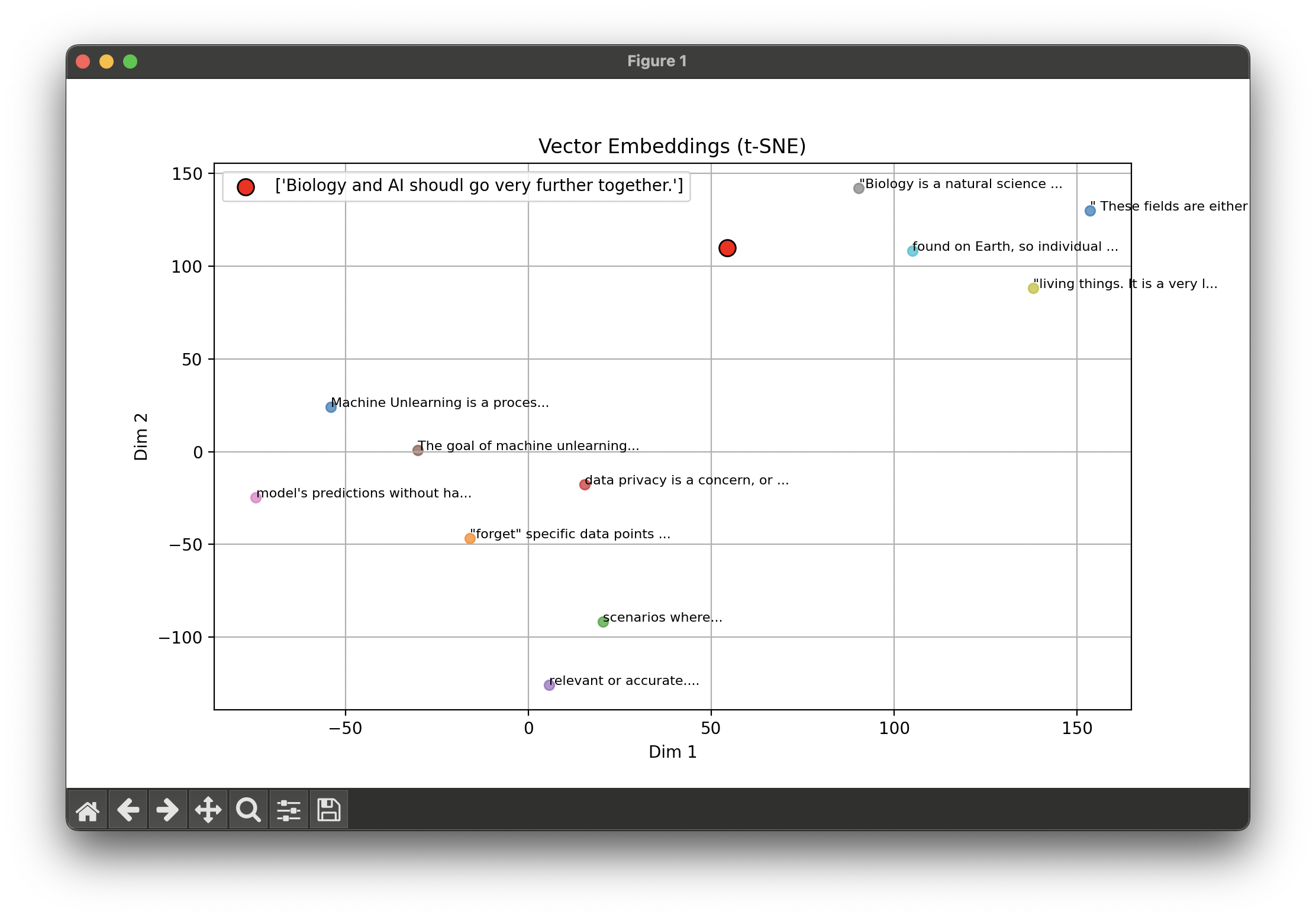
import matplotlib.pyplot as plt
from sklearn.manifold import TSNE
from sklearn.decomposition import PCA

query_embedding = model.encode(query_texts)

data = collection.get(include=["embeddings", "metadatas", "documents"])
embeddings = data["embeddings"]

# Use document text snippets as labels instead of source metadata
labels = [doc[:30] + "..." for doc in data["documents"]]

# Combine embeddings
all_embeddings = np.vstack([embeddings, query_embedding])
all_labels = labels + ["QUERY"]

# Reduce dimensions
reducer = TSNE(n_components=2, perplexity=5, random_state=42)
reduced = reducer.fit_transform(all_embeddings)

# Plot
plt.figure(figsize=(10, 6))
for i, (x, y) in enumerate(reduced[:-1]):
    plt.scatter(x, y, alpha=0.7)
    plt.text(x + 0.01, y + 0.01, labels[i], fontsize=8)

plt.scatter(
    reduced[-1][0], reduced[-1][1], color='red', label=query_texts[:30], s=100, edgecolor='black'
)
plt.title("Vector Embeddings (t-SNE)")
plt.xlabel("Dim 1")
plt.ylabel("Dim 2")
plt.grid(True)
plt.legend()
plt.show()

Key Considerations:

• Indexing Parameters: Tuning parameters like efConstruction, M (HNSW) or nlist, nprobe (IVF) impacts the speed/accuracy trade-off.
• Distance Metric: Common choices are Cosine Similarity (cosine), Euclidean Distance (l2), or Inner Product (ip). Cosine is often preferred for text embeddings as it measures orientation regardless of magnitude. Ensure your chosen metric aligns with how your embedding model was trained.
• Metadata Filtering: Effective use of metadata filters (where clause in ChromaDB example) can significantly narrow down the search space before the ANN search, improving relevance and speed.
• Scalability & Cost: Consider your data size, query volume, and latency requirements when choosing between local libraries, self-hosted databases, or managed services.

We also added a part to show the embedding and query together for visualization.

Changing the chunk size result in different embeddings samples which can be observed to understand its effects.

5. Semantic Search Mechanics

We’ve stored our document chunks as vectors in a specialized database. Now, how does the “Retrieval” part of RAG actually work? How do we take a user’s query, also represented as a vector, and efficiently find the most relevant document chunks from our vast collection? This is the domain of Semantic Search.

Beyond Keywords: The Semantic Leap

Traditional search engines often rely heavily on keywords. They find documents containing the exact words (or variations like stems) present in the query. This works well for specific terms but struggles with understanding intent or meaning.

Semantic Search, powered by embeddings, overcomes this. It focuses on the semantic relationship between the query and the documents.

• Query: “What are the best ways to travel from London to Paris?”
• Keyword Search Might Miss: Documents mentioning “Eurostar,” “Chunnel,” “flights between LHR and CDG,” or “driving across the channel” if they don’t contain the exact query words.
• Semantic Search Should Find: Documents discussing these travel methods because their meaning (and thus their embeddings) are related to the query’s meaning.

The Core Process:

1. Embed the Query: The user’s input query is processed using the exact same embedding model that was used to embed the document chunks. This is crucial! Using different models would place the query vector in an incompatible space.
2. Vector Similarity Search: The query_embedding is sent to the vector database (which we set up in the previous step). The database uses its ANN index (e.g., HNSW, IVF) to efficiently find the k vectors (document chunk embeddings) in its index that are “closest” to the query_embedding.

The Output: At the end of this stage, we have a list of text chunks deemed most relevant to the user’s query according to semantic similarity. These retrieved snippets are the “R” (Retrieval) in RAG. They form the crucial context that will be passed to the LLM in the next step to “Augment” the generation process.

Next, we’ll explore how to effectively combine this retrieved context with the original query to guide the LLM’s generation.