Attention:
Attention is one of the most talked about thing which became popular after the paper Attention is all you need. To talk about the high overview of attention, it is all about the values that gives importance to some of the part than others in this case. We will try our hands on attempt to code self attention from scratch today. Before starting, lets take a step back and understand how attention comes into place at all.
The problem with modeling long sequences
In an encoder-decoder RNN, the input text is fed into the encoder, which processes it sequentially. The encoder updates its hidden state at each step, trying to capture the entire meaning of input sequence in the final hidden state, The decoder then takes this final hidden state to start generating the translated sentence, one word at a time. It also updates its hidden state at each step, which is supposed to carry the context necessary for the next-word prediction.
You can see what seems like an issue here. To represent the whole information, encoder part processes the entire input text to hidden state. Since no access to earlier hidden state but only the present state, this could lead to the loss of context - especially in complex or long sentences.
Bahdanau’s attention mechanism provided a simple means by which the decoder could dynamically attend to different parts of the input at each decoding step. The high-level idea is that the encoder could produce a representation of length equal to the original input sequence. Then, at decoding time, the decoder can (via some control mechanism) receive as input a context vector consisting of a weighted sum of the representations on the input at each time step. This helped in capturing data dependencies.
Three years later, researchers found that RNN architectures are not required for building deep neural networks for NLP and proposed original transformer architecture with a self attention mechanism inspired b Bahdanau.
Self-attention:
Self-attention is a mechanism that helps a model focus on different parts of the same input sequence when processing each element. In self-attention, the “self" refers to the mechanism’s ability to compute attention weights by relating different positions within a single input sequence.
At the end of this blog, we should be able to define a self-attention module like this while understanding how it works from scratch.
import torch.nn as nn
class SelfAttention(nn.Module):
    def __init__(self, d_in, d_out,qkv_bias=False):
        super().__init__()
        self.d_out = d_out

        self.W_q = nn.Linear(d_in, d_out, bias=qkv_bias)
        self.W_k = nn.Linear(d_in,d_out, bias=qkv_bias)
        self.W_v = nn.Linear(d_in,d_out, bias=qkv_bias)

    def forward(self,X):
        """
        X: input tensor of shape ( seq_len, d_in)
        """
        query =self.W_q(X)
        key = self.W_k(X)
        value =self.W_v(X)

        attention_scores = query @ key.T
        attention_weights = torch.nn.functional.softmax(attention_scores/ self.d_out **0.5, dim=-1)
        context_vector = attention_weights @ value
        return context_vector
So, lets understand step by step. Starting with the simplified version of self-attention we will at the end implement the self-attention mechanism with trainable weights.
Self-attention mechanism without trainable weights
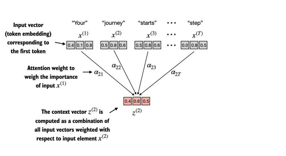
Consider the given figure, We would have input sequence as x consisting of T elements. For simplicity, we would consider an example of Your journey starts with one step as input sequence x. Each token would be represented by their embedding vector of dimension d. In our case, each token is being represented by three dimensional embedding vector.
Our goal is to calculate context vectors Z⁽ᶦ⁾ for each element X⁽ᶦ⁾.
In this example, first we will illustrate how we can obtain the context vector for x(2) i.e. journey word.
Lets first define the inputs as per the figure above. The input shape is 6 x 3 where 3 is the embedding dimension.
import torch
inputs = torch.tensor(
[[0.43, 0.15, 0.89], # Your (x^1)
[0.55, 0.87, 0.66], # journey (x^2)
[0.57, 0.85, 0.64], # starts (x^3)
[0.22, 0.58, 0.33], # with (x^4)
[0.77, 0.25, 0.10], # one (x^5)
[0.05, 0.80, 0.55]] # step (x^6)
)
In order to find the context vector for x(2), first we would calculate the attention score between query x(2) and all other input elements as a dot product. So, if i had to find the context vector for x(1), the query would be x(1) and attention score would be calculate between all other input elements as dot product.
query = inputs[1] # journey's embeddings
attention_scores_2 = torch.zeros(inputs.shape[0])
for i,x_i in enumerate(inputs):
	attention_scores_2[i] = torch.dot(x_i,query)
print(attention_scores_2)
The attention score is the normalized to obtain the attention weights that sums upto 1. By normalizing, we:
- Ensure the sum of attention scores is 1, treating them as probability-like weights.
- Maintain consistency across different sequences and input sizes.
- Prevent excessive dominance of certain values, leading to better learning.
Softmax is the most common normalization method in self-attention because it converts raw scores into a probability distribution while preserving relative importance. In practice , Softmax is preferred in self-attention as it handles extreme values and ensures smooth gradient propagation during training.
attention_weights_2 = torch.softmax(attention_scores_2,dim=0)
Now, we can calculate the context vector Z(2) by combining all the input vectors weighted by attention weights.
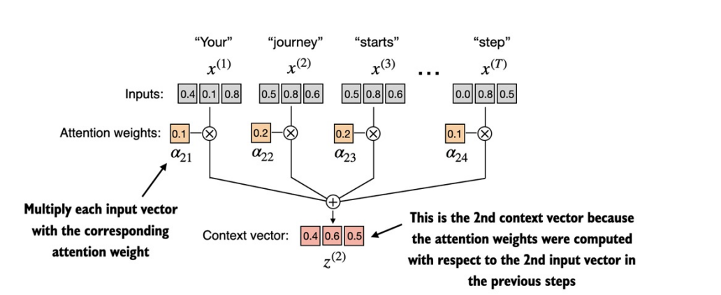
Implementing it in a code:
query = inputs[1] # 2nd input token is the query
context_vec_2 = torch.zeros(query.shape)
for i,x_i in enumerate(inputs):
	context_vec_2 += attn_weights_2[i]*x_i
print(context_vec_2)
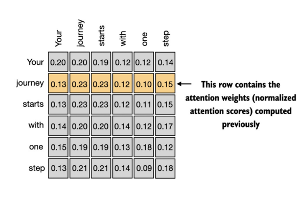
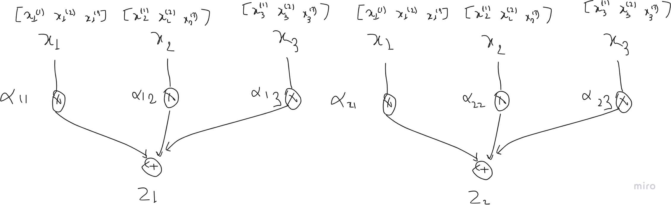
Computing attention weights for all input tokens
While calculating the attention weights using query as x(2), we obtained, alpha21,alpha22,alpha23.. alpha26. Now For all input tokens, we can calculate the attention scores by using matrix multiplication as below:
attention_scores = torch.matmul(input, input.T)
print("Attention Scores:\n",attention_scores)

attention_weights = torch.softmax(attention_scores, dim=1)
print("Attention Weights:\n",attention_weights)
What we obtained is the attention weights of all the input tokens. The value should be similar to the given table if you’ve supposed the same input embedding at the beginnigs.
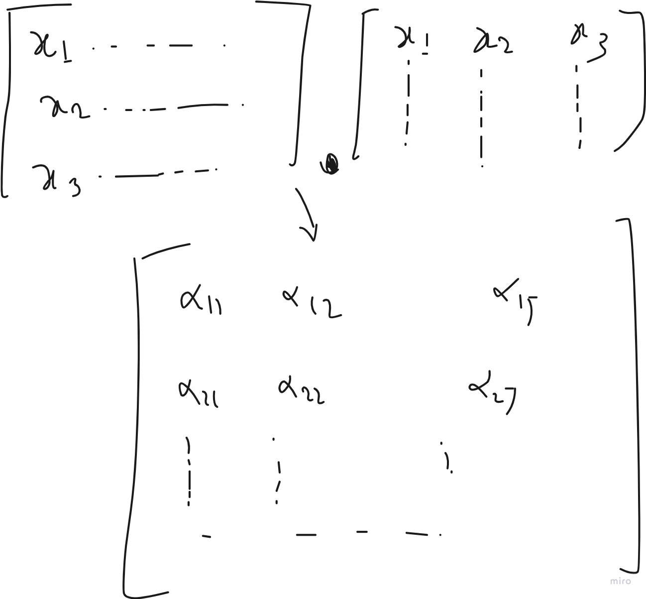
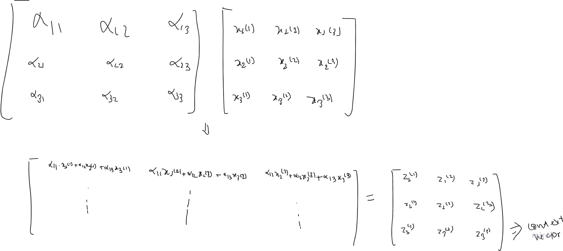
The final step is to calculate the context vector of each token. Since we obtained the attention weight matrix. We can simply matrix multiply over the inputs in order to obtain the same result for each token in a single time.
all_context_vecs = attn_weights @ inputs
print(all_context_vecs)
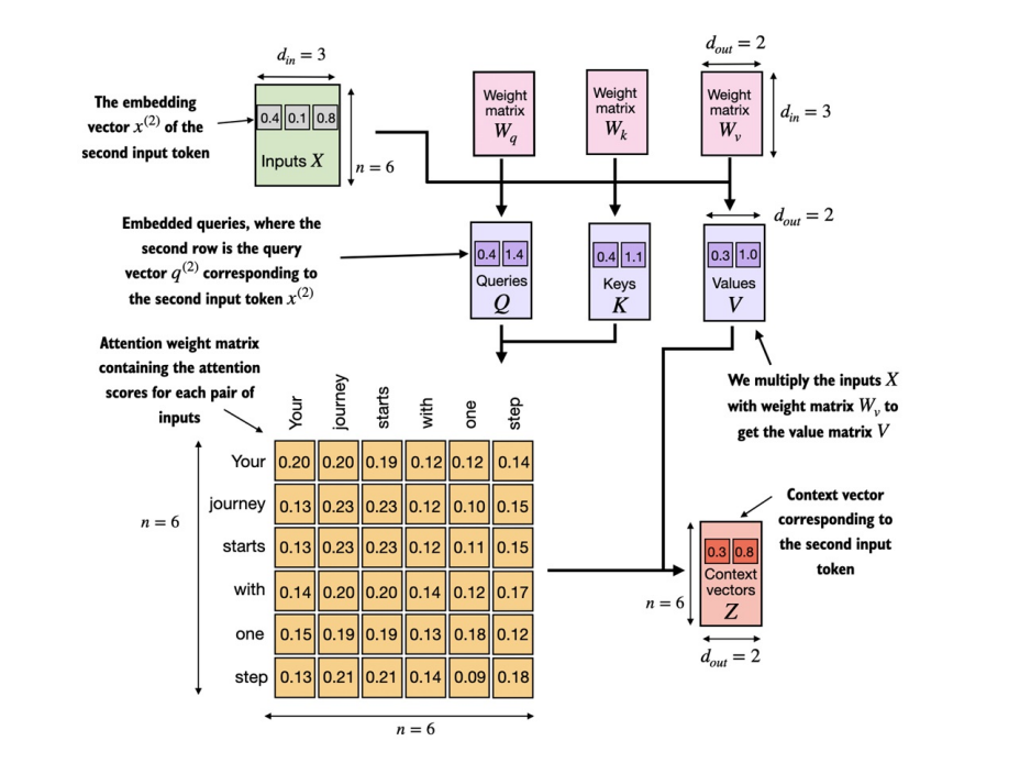
If you need to visualize yourself, how we are obtaining context vector with matrix multiplication, you can simply refer to the figure below which explains how individual context vector Z are being obtained and how matrix multiplication ease the process.
Self-attention with trainable weights
This self-attention mechanism is used in the original transformer architecture. This self-attention mechanism is also called scaled dot-product attention. We will get into that in a few time. The understanding of calculating the attention is almost identical, what really differs is the use of Weight matrices to obtain query , key and value from input tokens. These weight matrices are updated during model training so that model can learn to produce good context vectors.
Let’s start by coding step-by-step as before first.
We have to introduce three weight matrices Wq, Wv, Wk. These matrices are used to project input embedding into query, values and key respectively.
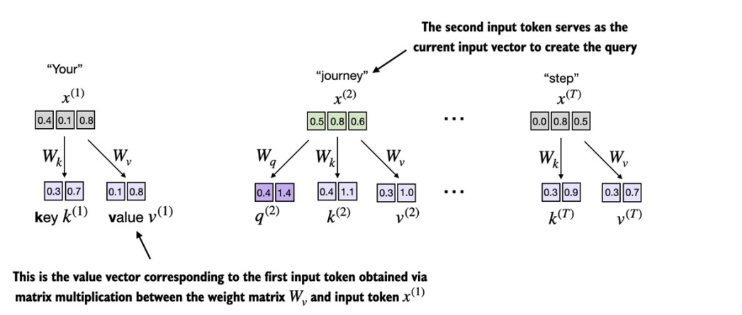
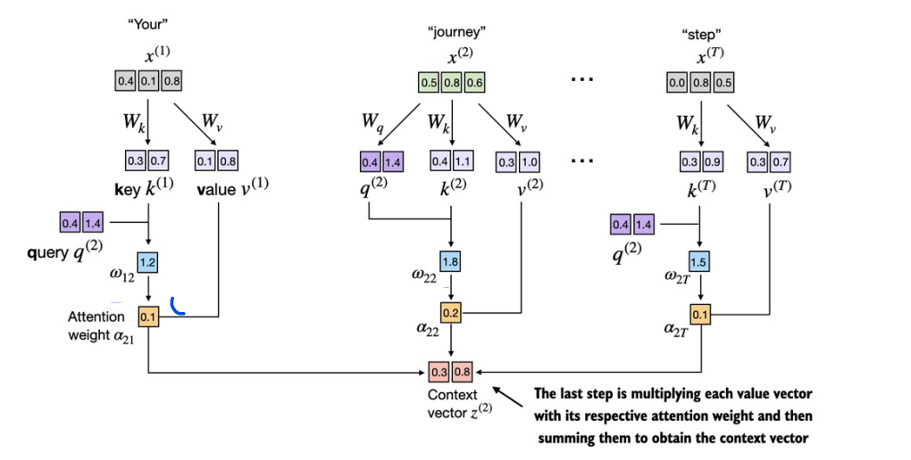
Just like earlier, we will first obtain context vector for input x2 i.e. “journey”. In order to obtain the attention weights for journey with all the other inputs, we need to obtain query for journey while key and value for all other tokens including itself.
X_2 = inputs[1]
d_in = inputs.shape[1] # embedding dimension of input
d_out = 2 # in some model like GPT, d_in = d_out
We now initialize three weight matrices Wq, Wk, and Wv as shown in figure above.
torch.manual_seed(123)
W_k = torch.nn.Parameter(torch.randn(d_in, d_out))
W_q = torch.nn.Parameter(torch.randn(d_in, d_out))
W_v = torch.nn.Parameter(torch.randn(d_in, d_out))
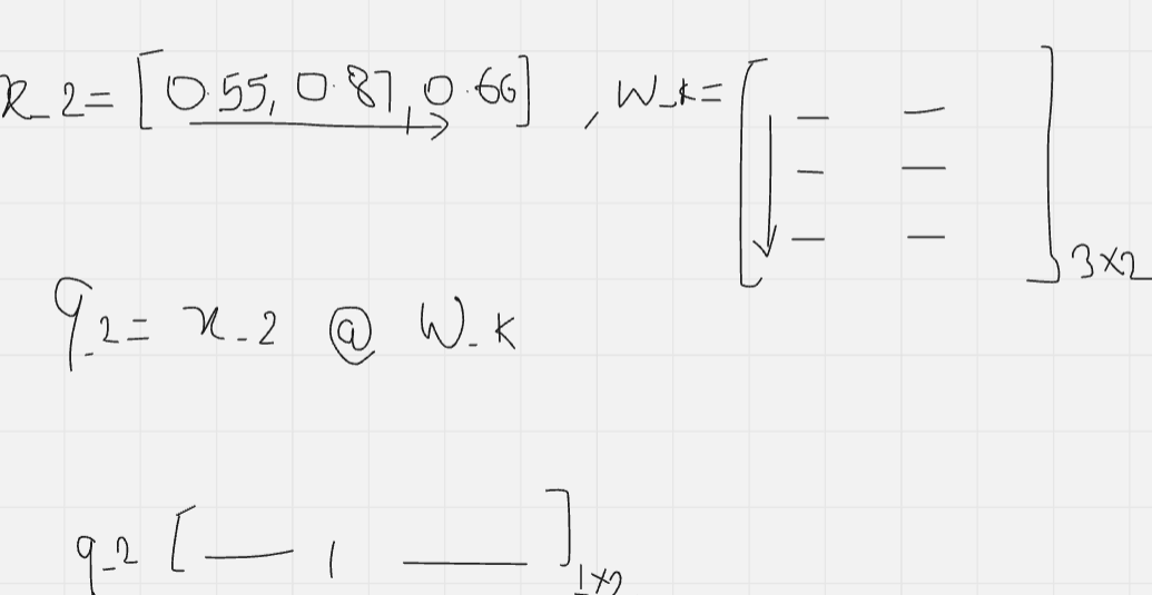
This basically project the x_2 into query, key and value into the shape of (1 x d_out)
query_2 = X_2 @ W_q
key_2 = X_2 @ W_k
value_2 = X_2 @ W_v
In order to obtain attention scores for x_2, we should obtain w_21, w_22, w_23, w_24 which refers to the attention scores of query 2 with keys of all respective tokens.
w_21 = torch.dot(query_2, keys[0])
w_22 = torch.dot(query_2, keys[1])
w_23 = torch.dot(query_2, keys[2])
w_24 = torch.dot(query_2, keys[3])
print(w_21, w_22, w_23, w_24)
Even though our temporary goal is to only compute the one context vector, z(2) , we still require the key and value vectors for all input elements as they are involved in computing the attention weights with respect to the query q(2)
keys = inputs @ W_key
values = inputs @ W_value
print("keys.shape:", keys.shape)
print("values.shape:", values.shape)
Lets compute attention scores w_22.
keys_2 = keys[1]
w_22 =  query_2.dot(keys_2)
print("W_22:",w_22)
To compute all the attention scores for x_2 via matrix muliplication, We can obtain these values with the same logic as mentioned in Computing attention weights for all input tokens without trainable weights section above. There we used matrix multiplication of input with its Transpose. In our case, we would take input as query and obtain the weights by multiplying with keys instead.
w_2 = query_2 @ keys.T
print(w_2)
Next step is to obtain attention weights by normalizing the attention scores. Remember, we talked about scaled dot attention earlier.
The rationale behind scaled-dot product attention: The reason for the normalization by the embedding dimension size is to improve the training performance by avoiding small gradients. For instance, when scaling up the embedding dimension, which is typically greater than thousand for GPT-like LLMs, large dot products can result in very small gradients during backpropagation due to the softmax function applied to them. As dot products increase, the softmax function behaves more like a step function, resulting in gradients nearing zero. These small gradients can drastically slow down learning or cause training to stagnate.
d_k = keys.shape[-1]
attn_weights_2 = torch.softmax(w_2 / d_k**0.5, dim=-1)
print(attn_weights_2)
Similar to earlier section where we computed the context vector as a weighted sum over the input vectors, we now compute the context vector as a weighted sum over the value vectors
context_vec_2 = attn_weights_2 @ values
print(context_vec_2)
Implementing a compact self-attention Python class
import torch.nn as nn
class SelfAttention(nn.Module):
    def __init__(self, d_in, d_out,qkv_bias=False):
        super().__init__()
        self.d_out = d_out

        self.W_q = nn.Linear(d_in, d_out, bias=qkv_bias)
        self.W_k = nn.Linear(d_in,d_out, bias=qkv_bias)
        self.W_v = nn.Linear(d_in,d_out, bias=qkv_bias)

    def forward(self,X):
        """
        X: input tensor of shape ( seq_len, d_in)
        """
        query =self.W_q(X)
        key = self.W_k(X)
        value =self.W_v(X)

        attention_scores = query @ key.T
        attention_weights = torch.nn.functional.softmax(attention_scores/ self.d_out **0.5, dim=-1)
        context_vector = attention_weights @ value
        return context_vector
Instead of using nn.Parameters we used nn.Linear because, it facilitates matrix multiplication easily as well as provides a better initialization of weights for training stability. This compact process represents the whole idea of self-attention in transformers.
Reference: Build a Large Language Model (From Scratch) by Sebastian Raschka, https://sebastianraschka.com/books/