Deep neural networks rely on the backpropagation algorithm to train effectively. A crucial component of backpropagation is the calculation of gradients, which dictate how much the weights in the network should be updated. However, when the sigmoid activation function is used in hidden layers, it can lead to the vanishing gradient problem. In this post, we’ll focus on how gradients are calculated and why sigmoid makes them vanish in deep networks.
Gradients in Back Propagation
In backpropagation, gradients are computed using the chain rule. For a weight $w$ in a hidden layer, the gradient of the loss ( L ) with respect to the weights ( w ) is given by the chain rule: $$ \frac{\partial L}{\partial w} = \frac{\partial L}{\partial a} \cdot \frac{\partial a}{\partial z} \cdot \frac{\partial z}{\partial w} $$
- a = f(z) is the output of the activation function
- z = w . x + b is the input to the activation function, where x is the input and b is the bias.
For a network with multiple layers, this process is repeated for every layer. The gradient at each layer depends on the product of gradients from all subsequent layers. This is where the sigmoid activation function introduces problems.
The sigmoid activation function is defined as:
$$ σ(x) = \frac{1}{1 + e^{-x}} $$
It maps any input x to a value between 0 and 1, which makes it particularly useful in scenarios requiring a probabilistic interpretation (e.g., binary classification). However, this very property also introduces significant drawbacks:
Saturation in the Output Range
For large positive or negative inputs, the sigmoid function saturates—meaning its output approaches 1 or 0. In these regions, the derivative of the sigmoid function is close to zero.
$$ σ’(x) = σ(x)(1 - σ(x)) $$
If σ(x) is near 0 or 1, σ’(x) becomes very small, leading to vanishing gradients. This can be demonstrated mathematically:
$$ \lim_{x \to +\infty} σ’(x) = \lim_{x \to +\infty} σ(x)(1 - σ(x)) = 1 \cdot (1 - 1) = 0 $$
$$ \lim_{x \to -\infty} σ’(x) = \lim_{x \to -\infty} σ(x)(1 - σ(x)) = 0 \cdot (1 - 0) = 0 $$
In a deep network, the gradient for weights in earlier layers is computed as a product of derivatives from all subsequent layers. When sigmoid is used as the activation function, each derivative σ′(z) is typically a small value (e.g., less than 0.25). As gradients are propagated backward, they get multiplied repeatedly. As the layer increases, the product of small derivatives leads to exponentially smaller gradients, which effectively kills the gradient preventing meaningful updates to the weights in earlier layers.
To illustrate this in our code:
We will implement our own ActivationFunction class as base class and the use Sigmoid for now.
class ActivationFunction(nn.Module):

    def __init__(self):
        super().__init__()
        self.name = self.__class__.__name__
        self.config = {"name": self.name}

class Sigmoid(ActivationFunction):

    def forward(self,x):
        return 1/(1+torch.exp(x))
To visualize the activation function and the gradient of the sigmoid function, Here is the code snippet.
# visualise the activation functions with gradinet

def get_gradient(act_fn, x):
    """
    Compute the gradient of the activation function at specified positions.
    Parameters:
    act_fn (callable): The activation function (e.g., nn.ReLU, torch.sigmoid).
    x (torch.Tensor): The input tensor where gradients are to be computed.

    Returns:
    torch.Tensor: Gradients of the activation function with respect to the input tensor.
    """
    x = x.clone().requires_grad_()
    out = act_fn(x)
    out.sum().backward()  # Compute gradients via backpropagation
    return x.grad  # Return the computed gradients

def vis_act_fn(act_fn,ax,x):
    y = act_fn(x)
    y_grads = get_gradient(act_fn, x)
    x,y,y_grads = x.numpy(), y.numpy(), y_grads.cpu().numpy()

    ax.plot(x,y,linewidth = 2, label = "ActFn")
    ax.plot(x, y_grads, linewidth=2, label="Gradient")
    ax.legend()
    ax.set_title(act_fn.name)
x = torch.linspace(-5, 5, 1000) # Range on which we want to visualize the activation functions
fig, ax = plt.subplots(1,1)

vis_act_fn(Sigmoid(),ax,x)
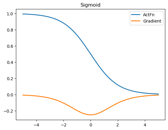
We can infer that if the input lies in saturation region, the gradient will be very close to zero. This leads to extremely small gradients during backpropagation.
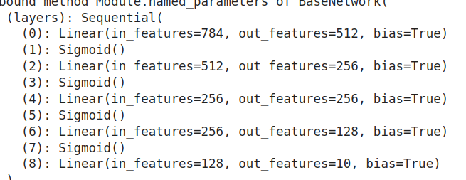
Consider a Neural Network Model as:
Code:
class BaseNetwork(nn.Module): def init(self,act_fn,input_size = 784, num_classes = 10, hidden_sizes = [512,256,256,128]):
class BaseNetwork(nn.Module):
    def __init__(self,act_fn,input_size = 784, num_classes = 10, hidden_sizes = [512,256,256,128]):

        super().__init__()

        # Create the network based on sp hidden sizes

        layers = []
        layer_sizes = [input_size] + hidden_sizes

        for layer_index in range(1, len(layer_sizes)):
            layers += [nn.Linear(layer_sizes[layer_index-1],layer_sizes[layer_index]), act_fn]
        layers += [nn.Linear(layer_sizes[-1],num_classes)]

        self.layers = nn.Sequential(*layers)

        # We store all hyperparameters in a dictionary for saving and loading of the model
        self.config = {"act_fn": act_fn.config, "input_size": input_size, "num_classes": num_classes, "hidden_sizes": hidden_sizes}

    def forward(self, x):
        x = x.view(x.size(0),-1)
        out = self.layers(x)
        return out
On visualizing the gradients of all the layers upon first batch passing through network, the computed gradients for the weights were visualized as:
def visualize_gradients(net, color="C0"):
    """
    Inputs:
        net - Object of class BaseNetwork
        color - Color in which we want to visualize the histogram (for easier separation of activation functions)
    """
    net.eval()
    small_loader = data.DataLoader(train_set, batch_size=256, shuffle=False)
    imgs, labels = next(iter(small_loader))
    imgs, labels = imgs.to(device), labels.to(device)

    # Pass one batch through the network, and calculate the gradients for the weights
    net.zero_grad()
    preds = net(imgs)
    loss = F.cross_entropy(preds, labels)
    loss.backward()
    # We limit our visualization to the weight parameters and exclude the bias to reduce the number of plots
    grads = {name: params.grad.data.view(-1).cpu().clone().numpy() for name, params in net.named_parameters() if "weight" in name}
    net.zero_grad()

    ## Plotting
    columns = len(grads)
    fig, ax = plt.subplots(1, columns, figsize=(columns*3.5, 2.5))
    fig_index = 0
    for key in grads:
        key_ax = ax[fig_index%columns]
        sns.histplot(data=grads[key], bins=30, ax=key_ax, color=color, kde=True)
        key_ax.set_title(str(key))
        key_ax.set_xlabel("Grad magnitude")
        fig_index += 1
    fig.suptitle(f"Gradient magnitude distribution for activation function {net.config['act_fn']['name']}", fontsize=14, y=1.05)
    fig.subplots_adjust(wspace=0.45)
    plt.show()
    plt.close()
To call the function:
net_actfn = BaseNetwork(Sigmoid()).to(device)
visualize_gradients(net_actfn,color=f"C2")

Observed Pattern:
-
Narrow Peaks Around Zero: Most gradients for deeper layers cluster near zero because sigmoid saturates for most inputs.
-
Slight Spread for Output Layer: Gradients in the final layers may show a broader distribution as they are closer to the loss function and receive stronger signals during backpropagation.
-
Gradient Diminution: As you move backward through the network (toward the input layer), the gradients shrink further.
-
Earlier Layers: Gradients are too small to effectively update the weights, leading to stagnation in learning.
-
Later Layers: Gradients remain relatively larger, so these layers can still learn meaningful representations.
The network becomes biased toward learning features in the later layers, while earlier layers remain under-trained. However, in classification problems, sigmoid is commonly used in the output layer for binary classification tasks:
Probability Interpretation: The sigmoid function σ(x) = 1 / (1 + e^(-x)) maps the final network output (logits) to a range between 0 and 1. This allows the output to be interpreted as a probability, which is essential for tasks like binary classification.
Alignment with Loss Functions: Sigmoid pairs well with the binary cross-entropy loss function. Together, they create a clear optimization goal:
$$ \text{Loss} = - \frac{1}{N} \sum_{i=1}^N \left[ y_i \log(\hat{y}_i) + (1 - y_i) \log(1 - \hat{y}_i) \right] $$
Here, ŷ_i (the predicted probability) comes directly from the sigmoid output.
To overcome Vanishing gradients there are other alternatives in practice such as:
- Use ReLU or its variants: These activations avoid saturation and maintain larger gradients, preventing vanishing gradients.
- Batch normalization: Helps keep activations within a range that avoids saturation.
- Residual connections (ResNets): Skip connections allow gradients to propagate more effectively through deeper networks.
Conclusion
Using the sigmoid activation function in the output layer is suitable for its probability interpretation in classification tasks and compatibility with cross-entropy loss. However, its limitations in the hidden layers, including saturation and vanishing gradients, make it unsuitable for deep networks. ReLU or its variants are better suited for hidden layers due to their robustness against these issues.
References
-
UVa Deep Learning Course Notebooks - Optimization and Initialization
Available at: [ Available at: https://uvadlc-notebooks.readthedocs.io/en/latest/tutorial_notebooks/tutorial3/Activation_Functions.html